Measuring and Simulating our Cheap Dielectric Probes

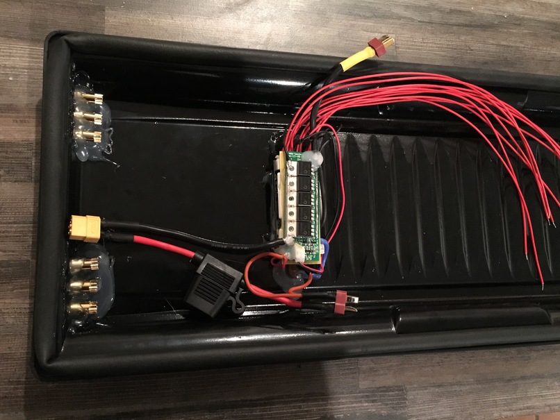
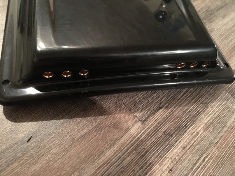
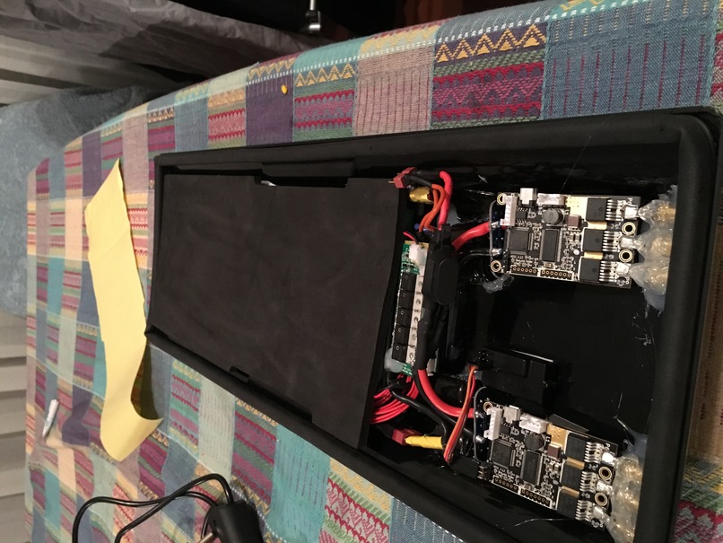
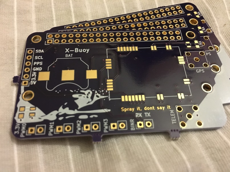
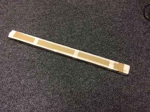
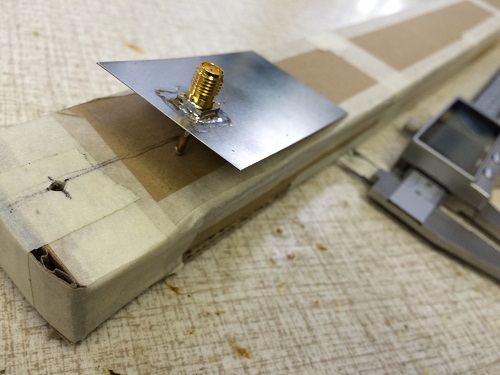
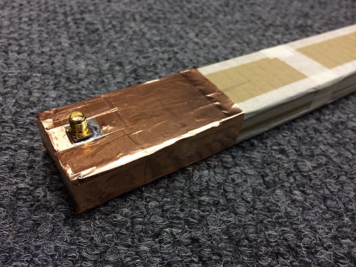
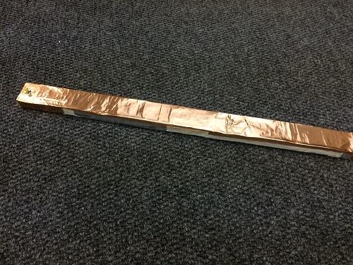
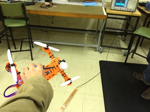
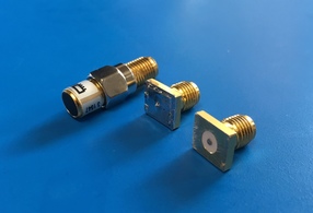
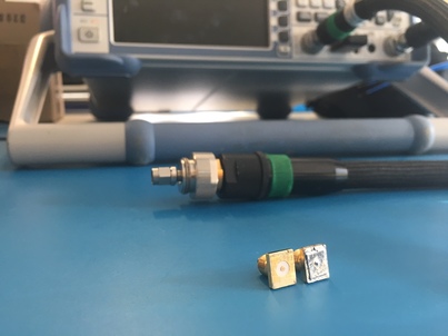
 As a follow up to my previous post, I built some simple SMA dielectric probes using PCB edge mount connectors. The probe interface surface is rather rough and the short was made using some soldered copper tape. This is definitely not the ideal set of probes. Nevertheless, I was curious how the probe would compare to its simulated counterpart. All of the dimensions were measured as accurately as possible using a set of digital callipers. The measurements were done on a VNA seen in the photo below.

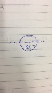
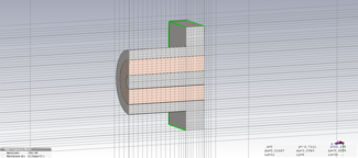
A cross-section of the mesh and model used in CST Microwave Office:

The rest of the post is the Jupyter Notebook that I used to analyse the measurements and simulation. I attempted to calibrate the probe parameters but still found too large of a difference between the measurement and simulation to use it in an actual permittivity extraction. In order to properly calibrate the probe, we definitely need a well-characterised reference material.


Probe Set Investigation

Import Measurement and Simulation data

In [58]:
# Define function to extract measurements data
import csv
import numpy as np
def read_s1p(filename):
    """
    Arguments:
    filename - filename including directory to measurement file.
    
    Returns
    freq - Measured frequency in Hz
    s11 - Measured scattering parameters in linear complex form 
    """
    freq = []
    s11 = []
    with open(filename, 'r') as csvfile:
        reader = csv.reader(csvfile, delimiter=' ', quotechar='|')
        for row in reader:
            row = list(filter(None, row))
            if len(row) == 3:
                freq.append(float(row[0]))
                s11.append(float(row[1]) + 1j*float(row[2]))
        freq = np.array(freq)
        s11 = np.array(s11)
        return freq, s11

Lets import all of our measurements and simulations using the read_s1p function

In [59]:
freq, s11_open = read_s1p("measurements/open.s1p")
freq, s11_short = read_s1p("measurements/short.s1p")
freq_cst, s11_open_cst = read_s1p("measurements/cst_open.s1p")
freq_cst, s11_short_cst = read_s1p("measurements/cst_short.s1p")
freq_cst, s11_open_cst_shifted = read_s1p("measurements/cst_open_shifted.s1p")
# Convert the CST frequency from GHz to Hz
freq_cst = freq_cst*1e9

Lets compare our probe-set measurements to their ideal simulation using CST Microwave Studio

In [60]:
import matplotlib.pyplot as plt

# Define S11 plotting function
def plt_s11(freq, s11):    
    plt.subplot(1, 2, 1)
    plt.plot(freq/1e6, 20*np.log10(np.abs(s11)))
    plt.plot(freq/1e6, 20*np.log10(np.abs(s11)))
    plt.xlim(freq[0]/1e6, freq[-1]/1e6)
    plt.ylim(-1,0.1)
    plt.xlabel("Freq [MHz]")
    plt.ylabel("S11 [dB]")
    plt.grid(True)
    plt.subplot(1, 2, 2)
    plt.plot(freq/1e6, np.angle(s11)*180/np.pi)
    plt.plot(freq/1e6, np.angle(s11)*180/np.pi)
    plt.xlim(freq[0]/1e6, freq[-1]/1e6)
    plt.ylim(-180,180)
    plt.xlabel("Freq [MHz]")
    plt.ylabel("S11 [Deg]")
    plt.grid(True)
    
# Plot Open
fig = plt.figure(figsize=(20, 4))
fig.suptitle("Open", fontsize=16)
plt_s11(freq, s11_open)
plt_s11(freq_cst, s11_open_cst)

# Plot Short
fig = plt.figure(figsize=(20, 4))
fig.suptitle("Short", fontsize=16)
plt_s11(freq, s11_short)
plt_s11(freq_cst, s11_short_cst)

plt.show()

The phase of both simulations match up well with their measurements. However, the short does have a substantial amount of loss across the entire band. This is most likely due to the copper tape that was used to create the short.

Shifting the Reference Plane to the Probe Interface

Using the open probe, which matched well with the simulation, we will add a phase offset to shift the reference plane from the connector to the probe interface.

In [61]:
l = 7.49e-3 # Distance from connector to probe interface
eps_r_teflon = 2.1 # Permittivity of teflon in coax
wavelength = 3e8/(freq)
vf = 1/np.sqrt(eps_r_teflon)
phase_offset = 2*np.pi*((2*l)/wavelength)/vf

# Apply the phase offset to all frequencies
s11_open_ref = s11_open*np.exp(1j*phase_offset)

# Plot the result compared to the simulated phase shifted result
fig = plt.figure(figsize=(20, 4))
fig.suptitle("Open Phase Shifted", fontsize=16)
plt_s11(freq, s11_open_ref)
plt_s11(freq_cst, s11_open_cst_shifted)
plt.ylim(-5,5)
plt.show()

Compared with the simulation the phase is about 1 degree off at the highest frequencies. This translates to geometrical errors in the submilimeter range. Polishing the end of the probe might improve this result.

Probe Capacitance and Radiating Conductance

Using the phase shifted measurement, we can calculate the probe calibration parameters.

In [62]:
e_c = 1 - 1j*0 # Permittfivity of a vacuum

# Define some parameters
w = 2*np.pi*freq
Z0 = 50
Y0 = 1/Z0

# Calculate the admittance of the air
Y = Y0*(1-s11_open_ref)/(1+s11_open_ref)

# Calculate the probe parameters
# Calculate A and B terms
A = 1j*w*e_c
B = np.power(e_c,5/2)

# Calculate the probe parameters
G_0 = (np.real(A)*np.imag(Y) - np.real(Y)*np.imag(A))/(np.real(A)*np.imag(B) - np.real(B)*np.imag(A))
C_0 = (np.imag(Y) - np.imag(B)*G_0)/np.imag(A)

# Plot the probe parameters 
fig = plt.figure(figsize=(20, 4))
plt.subplot(1, 2, 1)
plt.plot(freq/1e6, G_0)
plt.xlim(freq[0]/1e6, freq[-1]/1e6)
plt.xlabel("Freq [MHz]")
plt.ylabel("$G_0$")
plt.title("Radiating Conductance")
plt.grid(True)
plt.subplot(1, 2, 2)
plt.plot(freq/1e6, C_0)
plt.xlim(freq[0]/1e6, freq[-1]/1e6)
plt.xlabel("Freq [MHz]")
plt.ylabel("$C_0$")
plt.title("Fringing Capacitance")
plt.grid(True)
plt.show()
print("Fringing capacitance: "+str(np.average(C_0[1:])))
print("Radiating Conductance: "+str(np.average(G_0[1:])))
Fringing capacitance: 1.64635151707e-14
Radiating Conductance: 5.35396130766e-06

Measurement:
Fringing capacitance: 1.64773857969e-14
Radiating Conductance: 5.34207558123e-06

Simulation:
Fringing capacitance: 3.27689464957e-14
Radiating Conductance: 8.31421262357e-07

We find that only 1 degree in phase gives us double the fringing capacitance and almost 10 times less conductance. We are also ignoring losses in the short piece of coax transmission line in the probe. As a result, we really do need a good reference material to calibrate the probe. Just using a simulation and callipers will not be enough.

Dielectric Permittivity using a Coaxial Probe

Adding dielectric materials to electromagnetic simulations can be a pain if the correct dielectric properties are not known. To solve this I decided to build a poor-mans dielectric probe. The probe consists of a coaxial interface that is placed flush with a material under test. From a single reflection measurement of your material and a reference material, the complex permittivity can be calculated. As a first step, I simulated a probe with some dielectric materials and used the data to write and test my permittivity extraction code shown below. The procedure is common and can be found in multiple scientific papers.

The hardest part of the extraction is solving the 5th order polynomial. Because it was late in the evening, I opted for the brute force route and wrote a simple gradient decent algorithm to solve the complex permittivity.

The next step is to create the probe with some calibration standards and see if it works in practice.


Coaxial Probe Material Measurement and Calibration

Radim and Radislav: Broadband Measurement of Complex Permittivity
Using Reflection Method and Coaxial Probes

Set measured values and ref material parameters

In [270]:
# Measured Distilled Water
S11 = -0.097844 - 1j*0.99137
e_c = 78.4 + 1j*9.9762e-5

# Measured Teflon
S11_mut = 0.9983-1j*0.05831

Calulate admittance using S11

In [271]:
f = 1e9
w = 2*np.pi*f
Z0 = 50

Y0 = 1/Z0
Y = Y0*(1-S11)/(1+S11)
print("Admittance of distilled water: "+str(Y))
Admittance of distilled water: (8.473395759728993e-05+0.022070908693777157j)

Calculate probe capacitance parameters using distilled water measurement, $\epsilon_c$ is known.

\begin{equation*}
Y = j \omega \epsilon_c C_0 + \sqrt{\epsilon^5_c} G_0
\end{equation*}

To keep things clean, lets define:
\begin{equation*}
A = j \omega \epsilon_c \\\\
B = \sqrt{\epsilon^5_c}
\end{equation*}

Then we can calculate the probe parameters using:
\begin{equation*}
G_0 = \frac{Re(A)Im(Y) – Re(Y)Im(A)}{Re(A)Im(B) – Re(B)Im(A)}
\end{equation*}
\begin{equation*}
C_0 = \frac{Im(Y) – Im(B) G_0}{Im(A)}
\end{equation*}

In [272]:
import numpy as np

# Calculate A and B terms
A = 1j*w*e_c
B = np.power(e_c,5/2)

# Calculate the probe parameters
G_0 = (np.real(A)*np.imag(Y) - np.real(Y)*np.imag(A))/(np.real(A)*np.imag(B) - np.real(B)*np.imag(A))
C_0 = (np.imag(Y) - np.imag(B)*G_0)/np.imag(A)

print("C0: "+str(C0))
print("G0: "+str(G0))
C0: 4.48047731779e-14
G0: 1.55692371696e-09

Calculate admittance of MUT

In [273]:
Y_mut = Y0*(1-S11_mut)/(1+S11_mut)
print("Admittance of MUT: "+str(Y_mut))
Admittance of MUT: (-1.474302070865214e-08+0.0005835956264497135j)

Calculate the permittivity of the MUT using the probe parameters calculated earlier.

The equation is a 5th order polynomial which does not have any easy solutions. In order to save time, a simple gradient decent algorithm has been implemented to find the complex permittivity.

In [284]:
D = 1j*w*C_0

# Use gradient decent on this 2D space to calculate the complex permittivity
# Initialise permittivity (this should be your best guess)
e_mut = 1 + 0*1j
# Start loop
loss = [np.abs((D*e_mut + np.power(e_mut, 5/2)*G_0 - Y_mut))]
a = loss[-1]
count = 0
while loss[-1] > 1e-12:
    # Calculate derivatives
    rp = np.abs((D*(e_mut + a) + np.power(e_mut + a, 5/2)*G_0 - Y_mut))
    rn = np.abs((D*(e_mut - a) + np.power(e_mut - a, 5/2)*G_0 - Y_mut))
    ip = np.abs((D*(e_mut + a*1j) + np.power(e_mut + a*1j, 5/2)*G_0 - Y_mut))
    ine = np.abs((D*(e_mut - a*1j) + np.power(e_mut - a*1j, 5/2)*G_0 - Y_mut))

    # Calculate next point
    directions = np.array([rp, rn, ip, ine])
    steps = np.array([a, -a, a*1j, - a*1j])
    step = steps[directions - np.min(directions) == 0]
    e_mut = e_mut + step
    e_mut = e_mut[0]
    
    loss.append(np.abs((D*e_mut + np.power(e_mut, 5/2)*G_0 - Y_mut)))  
    a = 1000*np.abs(loss[-1])
    count += 1
print("Loss: "+str(loss[-1]))  
print("Iterations:"+str(count)) 
print("")    
print("E' : "+str(np.real(e_mut)))  
print("E'': "+str(np.imag(e_mut))) 
print("Loss tangent: "+str(np.imag(e_mut)/np.real(e_mut)))
print("Conductivity: "+str(np.imag(e_mut)*w)+str("S/m")) 

plt.figure()
plt.plot(loss[1:])
plt.show()
Loss: 9.08241678757e-13
Iterations:76

E' : 2.0730409503586182
E'': 8.659979628088184e-05
Loss tangent: 4.17742815287e-05
Conductivity: 544122.567597S/m


Electric Skateboard

Early 2016 was the year Tesla started showing off their new Model 3 electric car. Unfortunately, my financial situation did not allow me to own such a vehicle. As a result, I settled for the next best thing, building an incredibly overpowered electric skateboard.

Most of the drive system was ordered as a kit from Enertion (based in Australia). The kit contained dual 6355 brushless dc motors. Both motors were controlled using the popular VESC. The battery was self-assembled out of 40 18650 25R Samsung cells in a 10s4p configuration. I used one of the battery boxes available at Enertion to create a clean build without too much effort. The deck itself was ordered locally.

Below are some photos of the build process:

I will be adding some indicator LEDs to the top of the board, so the grip tape had to go.

Assembled drive system

Hot glueing ESC banana-plug connectors in the battery box

Routing a slot for the neo-pixel LED strip

Added inserts to the deck for mounting the battery box

Soldering the Li-ion battery pack

Finished 10s4p Li-ion pack

ESC’s and battery pack installed in battery box

Sealing LED strip using clear silicone

Replacing grip tape, leaving thin slot for LED strip


The LED strip was controlled using an ESP8266. It indicates speed, voltage, current as well as wifi connectivity. The plan was to upload data to a website using an MQTT system. However, excitement took over, and nothing except riding the board was accomplished after this. Since finishing the build, I estimate a total travel distance of more than a 1000 km commuting to and from work. The next post should go into more detail about the LEDs strip with some code and hopefully a working telemetry uploading feature.


Intelligent Ski Buoy take 2

It has been two years since I have touched this project. However, it has lingered in the back of my mind ever since. The significant issues with the previous design were positioning accuracy, skier safety and propulsion. Two of these hurdles were due to over optimising cost in the prototyping stage, which I now realise was a mistake. With lessons learned the new prototype is being built without cost optimisation. I think we can accept that a robotic course will be more expensive than an anchored course.

The new design is drastically different. The shape is entirely spherical with pod thrusters mounted inside the sphere. The sphere itself will be cast out of silicone to reduce injuries. Currently, the sphere is 3D printed for prototyping purposes. Amazingly, it is waterproof. The positioning will be handled using RTK GPS, a major step up from our GPS only system. As a result, positioning accuracy should be around 10 cm, which is probably what you can expect for a tethered course. With the added computation load of the RTK system, every buoy will be controlled using a raspberry pi zero. Consequently, this means ten Linux systems are floating in the water while you are skiing. Finally, we are able to reduce the system to ten buoys by directing the boat using a heads-up display.

Below are some pictures detailing the progress thus far.

Concept drawing

CAD drawing using Fusion 360

3D Printing the design

Adding some pod thrusters. Using normal brushless outrunner motors. Currently using 4 motors, will most probably use 2 in the final design to save cost.

Adding motor drivers and power distribution. Here things start to deviate from the CAD model. Nevertheless, this is a prototype and the main goal is to test the propulsion and station keeping.

PCB boards for RTK GPS, telemetry and breakout pins for the PWM pins. These boards are basically a hat for the raspberry pi.

In the next post, I will report back on the first propulsion test.


Homemade Waveguide Antenna for FPV Racing Timing Gate

In the past few years, FPV racing has quickly grown into a competitive sport. As a result, it has become necessary to keep track of lap times. Time-keeping is usually done using IR transmitters and receivers. However, this timing can be done without adding extra IR or RF beacons. By making use of the already present video transmitter on each vehicle, it is possible to keep track of every everyone in the race using their specific video channel frequency. However, there are some problems associated with using the 5.8 GHz emissions to track the vehicles. The first is the spatial accuracy where a timing event is triggered; the second is the effort needed to monitor the full FPV RF band continuously. The first problem in realising such a system is to design the receiving antenna.

A straightforward and cheap solution exists for the antenna. Using some cardboard, foil and aluminium or copper tape it is possible to build a high-gain waveguide antenna at 5.8 GHz. A slotted waveguide antenna has a thin disc shape antenna pattern which is ideally suited for use as a timing gate. Below are some photos showing the construction of the antenna.

Cardboard structure

Cardboard structure

Adding the feed structure

Adding the feed structure

Feed in place

Feed in place

Wrapping the rest of the waveguide in foil

Wrapping the rest of the waveguide in foil

Cutting waveguide slots

Cutting waveguide slots

Testing the antenna

Testing the antenna

The receiver needs to be broadband to be able to monitor all of the vehicles at the same time. For this, I would suggest mixing down the antenna signal to below 1 GHz and use multiple RTL-SDR dongles as a low-cost solution for monitoring all of the multi-copters in real-time.

Unfortunately, I have run out of time to work on the receiver. I will upload further data if there is interest in reproducing the antenna or continuing the project.

FPV Quadcopter Racing

After slipping into the world of quadcopters a few years ago, mostly for research purposes, I recently stumbled across a sport called FPV racing. This activity most commonly involves a small quadcopter equipped with a forward facing camera. The pilot then straps a monitor to his face and attempts to fly a designated race track. Think Red Bull Air racing, less expensive and less dangerous.

I built a 3D printed quadcopter based on the MHQ 2.0 on Thingiverse. All of the electronics were sourced from bandgood.com which made this probably the cheapest racer on the planet. Instead of buying the expensive Fatshark FPV goggles, I equipped myself with a Boscam transmitter and receiver along with Quanum foam goggles (Poor mans FPV option). In the end, I became comfortable with this setup with no regrets.

Yesterday I took part in the first race of the first official FPV racing competition in South Africa. My 3D printed underdog even made it past the first heat.

Below are some photos of my 3D printed FPV quad and South Africa first historical FPV race:

Pilots flying Race start image2

Smug face after coming second in my first heat.

The Intelligent Ski-Course

Last year I started building an intelligent ski-course, which was basically a set of buoy drones that would swim to there positions in a public river to form a ski course. This would then allow tons of interesting possibilities such as easy setup and effortlessly changing the shape of the course. Most of the project is documented on hackaday.io. As I am a very eager slalom skier in dire need of a course I would very much like to finish this project. However, I find myself without time working on finishing my PhD. I will one day restart my efforts, if anyone is interested in developing the project from where I left it, you are more that welcome, just keep me in the loop.

The state of the project:

  1. Most of the code has been written.
  2. The electronics for the buoy and base station has been mostly finalized
  3. 3D printed parts needs to be revised
  4. Propulsion system needs to be tested

Birth of FEMU 2.0

As part of my PhD research, involving the characterisation of the propagation environment at the SKA Karoo, time was spent developing a multi-copter RF metrology vehicle. A dramatic autopilot failure in our early prototype caused a the multi-copter to fly away forever. This event gave us a clean slate to do a full redesign upon what we have learned. One of the main problems with RF metrology using a multi-copter is the effect of the multi-copter itself on the measurement, which at this point has not been adequately addressed in research. Therefore, we set out to design a vehicle that could be appropriately de-embedded from a measurement.

The performance of antennas onboard these vehicles are in most cases unknown or assumed. These antennas have a specific characteristic pattern which could cause significant fluctuations in the measured signal, depending on its orientation. Even if the orientation was kept constant, the antenna patterns are sensitive to changes in metallic structures of the vehicle. An excellent example of this is the replacement of batteries after a flight. The replacement battery might have slightly different dimensions, position and will most certainly perturb some of the ubiquitous wires in the system.

Our approach was to shield all of the subsystems of the vehicle in a metallic enclosure. This shielding gave us a platform which had a predictable antenna pattern. Also, by closing the complex metallic environment, accurate antenna simulations have been made possible. Additionally, FEMU 2.0 also boasts a quasi-isotropic antenna pattern and a bandwidth of 260 MHz to 960MHz (See the paper for more information on this).

Hopefully, this will pave the way for RF metrology using multi-copters. If done correctly this could significantly speed up measurement time and deliver measurements that are spatially continuous. The entire vehicle has been constructed from 3D printed parts and local hardware supplies. The electronics, receiver and antenna systems can all be made available if another research group is interested in further developing the project.

Below are two images showing FEMU 2.0 during setup and measurement.

Setting up FEMU 2.0 before flight


Don’t Leave Me…

Since the last post, we have completed a year of successfully RF measurement campaigns. Sadly, the quadcopter featuring in the previous post (FEMU 1.0) underwent an autopilot failure during a measurement dry-run which caused it to fly straight up into the air until its battery died. It has never been seen since. This forced us to build FEMU 1.5 in 3 days. Being a temporary vehicle, FEMU 1.5 was decommissioned shortly after his first measurement campaign (25 flights). All this happened in the earlier part of the year and gave us the opportunity to do a complete redesign which will be discussed in the next post. This redesign formed a large part of my PhD degree and made attempts to break new ground in RF metrology using Multicopters.

Reward if found poster for the disappearance of FEMU 1.0

Reward if found poster for the disappearance of FEMU 1.0

This was also the start of our quest to 3D print antennas, see the 900 MHz antenna mounted at the bottom.

FEMU 1.5 with a 900 MHz antenna

FEMU 1.5 with a 900 MHz antenna

My 3D Printer

I decided it would be a good idea for our lab, and for me, to have a 3D printer at our hands. After some consideration, I ordered a kit from a local supplier DIY Electronics whom I would gladly recommend. The kit, a relatively new design, is named a Prusa i3. Up to now, after the printer has been assembled and improved. I have yet to decide on a proper name.

Below is a very crude time lapse I made using my GoPro 3, suction-cupped against the wall.

After installing the Repetier host and firmware and getting the end stops and motors working in the correct directions I was able to successfully print a cube. Which I thought was way too easy. After some numerous calibration guides and models from Thingiverse I have calibrated my machine enough to print its own parts. The list of which I will share at the end of this post. He was originally just white, but now has a few black parts which were all self-printed with PLA.

printer2