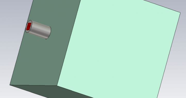
Adding dielectric materials to electromagnetic simulations can be a pain if the correct dielectric properties are not known. To solve this I decided to build a poor-mans dielectric probe. The probe consists of a coaxial interface that is placed flush with a material under test. From a single reflection measurement of your material and a reference material, the complex permittivity can be calculated. As a first step, I simulated a probe with some dielectric materials and used the data to write and test my permittivity extraction code shown below. The procedure is common and can be found in multiple scientific papers.
The hardest part of the extraction is solving the 5th order polynomial. Because it was late in the evening, I opted for the brute force route and wrote a simple gradient decent algorithm to solve the complex permittivity.
The next step is to create the probe with some calibration standards and see if it works in practice.
Coaxial Probe Material Measurement and Calibration
Radim and Radislav: Broadband Measurement of Complex Permittivity
Using Reflection Method and Coaxial Probes
Set measured values and ref material parameters
# Measured Distilled Water
S11 = -0.097844 - 1j*0.99137
e_c = 78.4 + 1j*9.9762e-5

# Measured Teflon
S11_mut = 0.9983-1j*0.05831
Calulate admittance using S11
f = 1e9
w = 2*np.pi*f
Z0 = 50

Y0 = 1/Z0
Y = Y0*(1-S11)/(1+S11)
print("Admittance of distilled water: "+str(Y))
Calculate probe capacitance parameters using distilled water measurement, $\epsilon_c$ is known.
\begin{equation*}
Y = j \omega \epsilon_c C_0 + \sqrt{\epsilon^5_c} G_0
\end{equation*}
To keep things clean, lets define:
\begin{equation*}
A = j \omega \epsilon_c \\\\
B = \sqrt{\epsilon^5_c}
\end{equation*}
Then we can calculate the probe parameters using:
\begin{equation*}
G_0 = \frac{Re(A)Im(Y) – Re(Y)Im(A)}{Re(A)Im(B) – Re(B)Im(A)}
\end{equation*}
\begin{equation*}
C_0 = \frac{Im(Y) – Im(B) G_0}{Im(A)}
\end{equation*}
import numpy as np

# Calculate A and B terms
A = 1j*w*e_c
B = np.power(e_c,5/2)

# Calculate the probe parameters
G_0 = (np.real(A)*np.imag(Y) - np.real(Y)*np.imag(A))/(np.real(A)*np.imag(B) - np.real(B)*np.imag(A))
C_0 = (np.imag(Y) - np.imag(B)*G_0)/np.imag(A)

print("C0: "+str(C0))
print("G0: "+str(G0))
Calculate admittance of MUT
Y_mut = Y0*(1-S11_mut)/(1+S11_mut)
print("Admittance of MUT: "+str(Y_mut))
Calculate the permittivity of the MUT using the probe parameters calculated earlier.
The equation is a 5th order polynomial which does not have any easy solutions. In order to save time, a simple gradient decent algorithm has been implemented to find the complex permittivity.
D = 1j*w*C_0

# Use gradient decent on this 2D space to calculate the complex permittivity
# Initialise permittivity (this should be your best guess)
e_mut = 1 + 0*1j
# Start loop
loss = [np.abs((D*e_mut + np.power(e_mut, 5/2)*G_0 - Y_mut))]
a = loss[-1]
count = 0
while loss[-1] > 1e-12:
    # Calculate derivatives
    rp = np.abs((D*(e_mut + a) + np.power(e_mut + a, 5/2)*G_0 - Y_mut))
    rn = np.abs((D*(e_mut - a) + np.power(e_mut - a, 5/2)*G_0 - Y_mut))
    ip = np.abs((D*(e_mut + a*1j) + np.power(e_mut + a*1j, 5/2)*G_0 - Y_mut))
    ine = np.abs((D*(e_mut - a*1j) + np.power(e_mut - a*1j, 5/2)*G_0 - Y_mut))

    # Calculate next point
    directions = np.array([rp, rn, ip, ine])
    steps = np.array([a, -a, a*1j, - a*1j])
    step = steps[directions - np.min(directions) == 0]
    e_mut = e_mut + step
    e_mut = e_mut[0]

    loss.append(np.abs((D*e_mut + np.power(e_mut, 5/2)*G_0 - Y_mut)))
    a = 1000*np.abs(loss[-1])
    count += 1
print("Loss: "+str(loss[-1]))
print("Iterations:"+str(count))
print("")
print("E' : "+str(np.real(e_mut)))
print("E'': "+str(np.imag(e_mut)))
print("Loss tangent: "+str(np.imag(e_mut)/np.real(e_mut)))
print("Conductivity: "+str(np.imag(e_mut)*w)+str("S/m"))

plt.figure()
plt.plot(loss[1:])
plt.show()

Pingback: Measuring and Simulating our Cheap Dielectric Probes – Hardie Pienaar