DIY Star Realms Counters

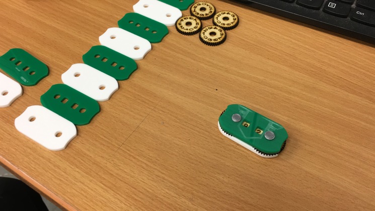
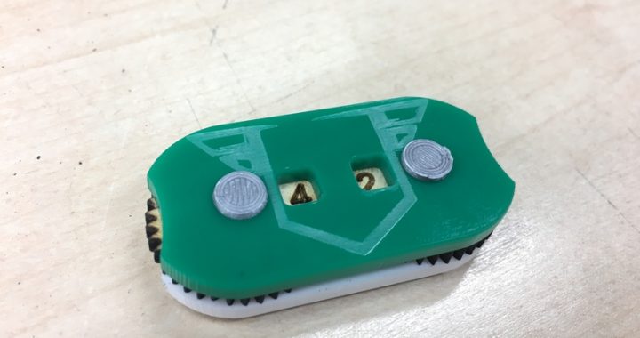
If you have ever played Star Realms before you may have noticed the interesting card counting system. In most cases, this system works well. However, after a beer or two results start to vary. I made some counter tokens for my set which worked surprisingly well. Counters only require average human maths. If you have access to a laser-cutter and 3D printer feel free to download the files below and make your own.

star_realms_counter


Vector Spherical Harmonic Python Tools for FEKO

I recently found myself in a situation where I needed to simulate many antenna configurations while storing all of their far-field patterns. The far-field patterns themselves are described on a spherical grid using, in my case, 26×101 points. That is more than 2000 data points per frequency. If you are simulating 60 frequency points, this explodes to around 150000 data points per antenna simulation. This is fine if you are running the odd few simulations. However, on this occasion, I was attempting to simulate an unwieldy set of 4000 different antenna configurations. This might be more simulations than most people run in an entire lifetime. Nevertheless, I was determined. Just to translate the problem into hard drive space, 150k times 4000 is around 600M data points. Keep in mind that this is not your average byte sized data points. Every data point is a complex vector leading to a dataset well into the Gigabyte ranges. For a mere RF engineer, this is some serious big data territory.

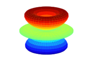
Thankfully, we can compress the far-field dataset with a handy tool called Vector Spherical Harmonics (VSH). FEKO allows you to export the VSH modes which for the typical antenna only involves around 200 data points that need to be stored compared to 2000 from before.

The reason I wrote this post is to share my python implementation of the VSH used in FEKO. You can grab the code from the GitHub link. The code itself allows you to plot the far-field from the complex mode coefficients given by FEKO. It also includes functions to extract these coefficients from the FEKO outfile. Feel free to send me pull requests to make this code better.

FEKO Parameter Sweep Lua Script

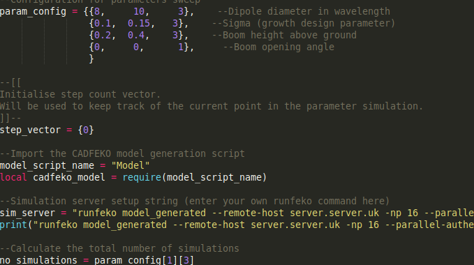
Part of my work at the Cavendish Laboratory involves optimisation of the SKA Low aperture array antenna. As a result, a substantial amount of FEKO gets used. During my efforts, I created a script that allows for parameter sweeps over a parameterised FEKO model over an arbitrary number of input dimensions. Using a Lua scripting built into CADFEKO, it is possible to generate geometries where structures can be added and removed. This comes in handy when you want to change the number of elements in your Yagi or LPDA antenna. I found this script extremely useful in optimising my antenna design and hope it can be of use to the larger FEKO community.

Usage:

The current script has 3 files:

  • Model.lua
  • parametersweep.lua
  • Parametric_Model_Source.cfx

Model.lua is your own antenna scripting file (add antenna here). I found the FEKO documentation (F1) very useful for finding functions that I needed. Use this file as an example to create your own antenna.

parametersweep.lua handles the loop process that generates the CADFEKO geometry from Model.lua and invokes runfeko to simulate the file. You might need to create a results folder on your machine for the script to copy the results into. During some experimentation, I also found it useful to call python scripts from the main loop to calculate metrics from the results.

Parameteric_Model_Source.cfx exists because I was too lazy to figure out how to add wire ports and voltage sources to the parametric antenna model. Nevertheless, this file is used to define your result requests and other simulation parameters like frequency, etc.

To start the script, open CADFEKO by opening the Parametric_Model_Source.cfx. Open the scripts editor from the ribbon bar. You need to careful here not to edit or use old scripts, FEKO reopens the last scripts that were used. For safety, I tend to close all the tabs and make sure I open the correct script. Finally with the parametersweep.lua file open, click the run command and get ready for some chaos on the screen.

If you have some improvements that you have added to your own script, let me know so that I can add it to this page. In its current state, it does not work on Linux or Mac. Also, during simulation, it will occasionally grab your mouse focus when it opens and closes the cmd window.

Download the script here

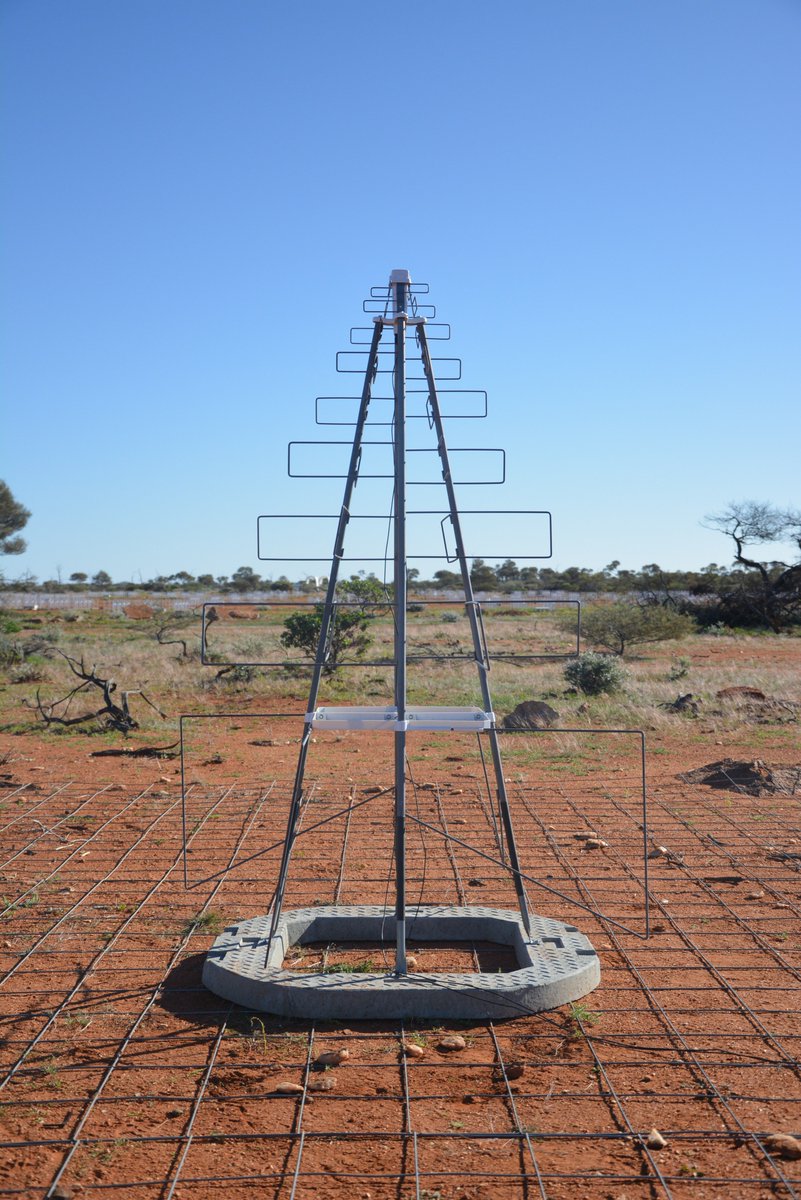
Remember, antennas should roam free. No antenna deserves to be caged and crammed into your smartwatch.

Example of an antenna in the wild (SKALA2 https://www.icrar.org/)
Measuring and Simulating our Cheap Dielectric Probes

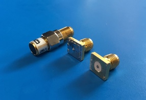
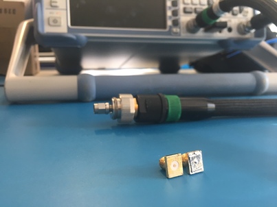
 As a follow up to my previous post, I built some simple SMA dielectric probes using PCB edge mount connectors. The probe interface surface is rather rough and the short was made using some soldered copper tape. This is definitely not the ideal set of probes. Nevertheless, I was curious how the probe would compare to its simulated counterpart. All of the dimensions were measured as accurately as possible using a set of digital callipers. The measurements were done on a VNA seen in the photo below.

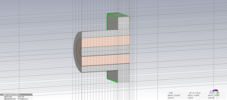
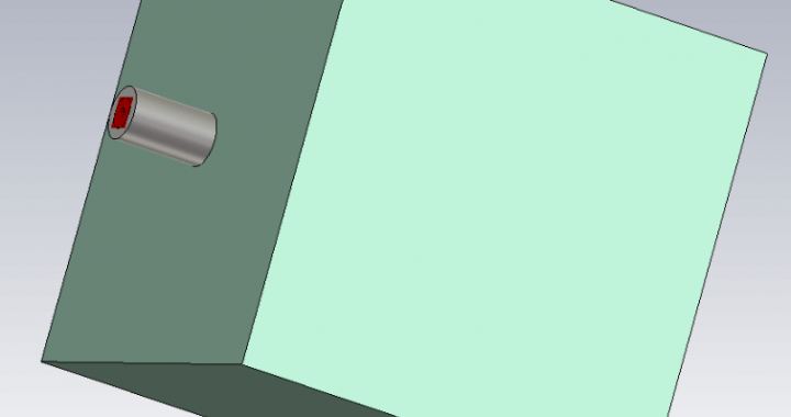
A cross-section of the mesh and model used in CST Microwave Office:

The rest of the post is the Jupyter Notebook that I used to analyse the measurements and simulation. I attempted to calibrate the probe parameters but still found too large of a difference between the measurement and simulation to use it in an actual permittivity extraction. In order to properly calibrate the probe, we definitely need a well-characterised reference material.


Probe Set Investigation

Import Measurement and Simulation data

In [58]:
# Define function to extract measurements data
import csv
import numpy as np
def read_s1p(filename):
    """
    Arguments:
    filename - filename including directory to measurement file.
    
    Returns
    freq - Measured frequency in Hz
    s11 - Measured scattering parameters in linear complex form 
    """
    freq = []
    s11 = []
    with open(filename, 'r') as csvfile:
        reader = csv.reader(csvfile, delimiter=' ', quotechar='|')
        for row in reader:
            row = list(filter(None, row))
            if len(row) == 3:
                freq.append(float(row[0]))
                s11.append(float(row[1]) + 1j*float(row[2]))
        freq = np.array(freq)
        s11 = np.array(s11)
        return freq, s11

Lets import all of our measurements and simulations using the read_s1p function

In [59]:
freq, s11_open = read_s1p("measurements/open.s1p")
freq, s11_short = read_s1p("measurements/short.s1p")
freq_cst, s11_open_cst = read_s1p("measurements/cst_open.s1p")
freq_cst, s11_short_cst = read_s1p("measurements/cst_short.s1p")
freq_cst, s11_open_cst_shifted = read_s1p("measurements/cst_open_shifted.s1p")
# Convert the CST frequency from GHz to Hz
freq_cst = freq_cst*1e9

Lets compare our probe-set measurements to their ideal simulation using CST Microwave Studio

In [60]:
import matplotlib.pyplot as plt

# Define S11 plotting function
def plt_s11(freq, s11):    
    plt.subplot(1, 2, 1)
    plt.plot(freq/1e6, 20*np.log10(np.abs(s11)))
    plt.plot(freq/1e6, 20*np.log10(np.abs(s11)))
    plt.xlim(freq[0]/1e6, freq[-1]/1e6)
    plt.ylim(-1,0.1)
    plt.xlabel("Freq [MHz]")
    plt.ylabel("S11 [dB]")
    plt.grid(True)
    plt.subplot(1, 2, 2)
    plt.plot(freq/1e6, np.angle(s11)*180/np.pi)
    plt.plot(freq/1e6, np.angle(s11)*180/np.pi)
    plt.xlim(freq[0]/1e6, freq[-1]/1e6)
    plt.ylim(-180,180)
    plt.xlabel("Freq [MHz]")
    plt.ylabel("S11 [Deg]")
    plt.grid(True)
    
# Plot Open
fig = plt.figure(figsize=(20, 4))
fig.suptitle("Open", fontsize=16)
plt_s11(freq, s11_open)
plt_s11(freq_cst, s11_open_cst)

# Plot Short
fig = plt.figure(figsize=(20, 4))
fig.suptitle("Short", fontsize=16)
plt_s11(freq, s11_short)
plt_s11(freq_cst, s11_short_cst)

plt.show()

The phase of both simulations match up well with their measurements. However, the short does have a substantial amount of loss across the entire band. This is most likely due to the copper tape that was used to create the short.

Shifting the Reference Plane to the Probe Interface

Using the open probe, which matched well with the simulation, we will add a phase offset to shift the reference plane from the connector to the probe interface.

In [61]:
l = 7.49e-3 # Distance from connector to probe interface
eps_r_teflon = 2.1 # Permittivity of teflon in coax
wavelength = 3e8/(freq)
vf = 1/np.sqrt(eps_r_teflon)
phase_offset = 2*np.pi*((2*l)/wavelength)/vf

# Apply the phase offset to all frequencies
s11_open_ref = s11_open*np.exp(1j*phase_offset)

# Plot the result compared to the simulated phase shifted result
fig = plt.figure(figsize=(20, 4))
fig.suptitle("Open Phase Shifted", fontsize=16)
plt_s11(freq, s11_open_ref)
plt_s11(freq_cst, s11_open_cst_shifted)
plt.ylim(-5,5)
plt.show()

Compared with the simulation the phase is about 1 degree off at the highest frequencies. This translates to geometrical errors in the submilimeter range. Polishing the end of the probe might improve this result.

Probe Capacitance and Radiating Conductance

Using the phase shifted measurement, we can calculate the probe calibration parameters.

In [62]:
e_c = 1 - 1j*0 # Permittfivity of a vacuum

# Define some parameters
w = 2*np.pi*freq
Z0 = 50
Y0 = 1/Z0

# Calculate the admittance of the air
Y = Y0*(1-s11_open_ref)/(1+s11_open_ref)

# Calculate the probe parameters
# Calculate A and B terms
A = 1j*w*e_c
B = np.power(e_c,5/2)

# Calculate the probe parameters
G_0 = (np.real(A)*np.imag(Y) - np.real(Y)*np.imag(A))/(np.real(A)*np.imag(B) - np.real(B)*np.imag(A))
C_0 = (np.imag(Y) - np.imag(B)*G_0)/np.imag(A)

# Plot the probe parameters 
fig = plt.figure(figsize=(20, 4))
plt.subplot(1, 2, 1)
plt.plot(freq/1e6, G_0)
plt.xlim(freq[0]/1e6, freq[-1]/1e6)
plt.xlabel("Freq [MHz]")
plt.ylabel("$G_0$")
plt.title("Radiating Conductance")
plt.grid(True)
plt.subplot(1, 2, 2)
plt.plot(freq/1e6, C_0)
plt.xlim(freq[0]/1e6, freq[-1]/1e6)
plt.xlabel("Freq [MHz]")
plt.ylabel("$C_0$")
plt.title("Fringing Capacitance")
plt.grid(True)
plt.show()
print("Fringing capacitance: "+str(np.average(C_0[1:])))
print("Radiating Conductance: "+str(np.average(G_0[1:])))
Fringing capacitance: 1.64635151707e-14
Radiating Conductance: 5.35396130766e-06

Measurement:
Fringing capacitance: 1.64773857969e-14
Radiating Conductance: 5.34207558123e-06

Simulation:
Fringing capacitance: 3.27689464957e-14
Radiating Conductance: 8.31421262357e-07

We find that only 1 degree in phase gives us double the fringing capacitance and almost 10 times less conductance. We are also ignoring losses in the short piece of coax transmission line in the probe. As a result, we really do need a good reference material to calibrate the probe. Just using a simulation and callipers will not be enough.

GUI Text Box in Terminal

Having a GUI in the terminal would be ”interesting”. Here is some code to display a box with a title and content. Its far from a GUI, but its a start. This idea might just be used in my autonomous buoy project for displaying telemetry data.

from colorama import Fore, Back, Style

def gen_text_box(title, size_x, size_y, content):
    """
    Arguments:
    title - Title string of box displayed at the top
    size_x - Horizontal character size of the box
    size_y - Vertical character size of the box
    content - String of content that needs to be displayed in the box

    Returns:
    line - string with box embedded, ready to be printed
    """
    
    BLANK_ROWS = 1
    BLANK_COL = 2

    t_start = int(size_x/2 - len(title)/2)
    t_stop = t_start + len(title)
    line = "" # Initialise drawing string to nothing

    # Draw top line
    for i in range(size_x):
        if i == 0:
            line = line + "\u250C"	
        elif i == size_x - 1:
            line = line + "\u2510"
        else:
            line = line + "\u2500"

    # Insert title
    start = line[0:t_start]
    end = line[t_stop:]
    line = Fore.CYAN+start+Fore.WHITE+title+Fore.CYAN+end # Make title white

    # Seperate content into an array of rows
    content_list = content.split('\n')

    # Draw side lines as well as content
    line = line + "\n"
    for i in range(size_y):
        c_line = ""
        for j in range(size_x):
            if j == 0:
                c_line = c_line + "\u2502"
            elif j == size_x-1:
                c_line = c_line + "\u2502"
            else:
                c_line = c_line + " "
        c_line = c_line + "\n"

        # Insert content line
        if i < len(content_list) + BLANK_ROWS and i > BLANK_ROWS-1:
            start = c_line[0:BLANK_COL]
            end = c_line[len(content_list[i-BLANK_ROWS]) + BLANK_COL:]
            c_line = Fore.CYAN+start+Fore.WHITE+content_list[i-BLANK_ROWS]+Fore.CYAN+end # Make title white
        line = line + c_line

    # Draw bottom line
    for i in range(size_x):
        if i == 0:
            line = line + "\u2514"	
        elif i == size_x - 1:
            line = line + "\u2518"
        else:
            line = line + "\u2500"
    line = line + "\n"
    return  line

# Earnings
monthly_earnings = 30000
daily_earnings = monthly_earnings/30.5
hourly_earnings = daily_earnings/8

# Want to spend
spend = 2500

# Calculations
days_work = round(spend/daily_earnings,3)
hourly_work = round(spend/hourly_earnings,2)

content = "Spending " + str(spend) + " amounts to: \n" +\
           str(hourly_work) + " hours of work \n" +\
           str(days_work) + " hard days of labour"

print(gen_text_box("Spendy", 40, 4, content))


Dielectric Permittivity using a Coaxial Probe

Adding dielectric materials to electromagnetic simulations can be a pain if the correct dielectric properties are not known. To solve this I decided to build a poor-mans dielectric probe. The probe consists of a coaxial interface that is placed flush with a material under test. From a single reflection measurement of your material and a reference material, the complex permittivity can be calculated. As a first step, I simulated a probe with some dielectric materials and used the data to write and test my permittivity extraction code shown below. The procedure is common and can be found in multiple scientific papers.

The hardest part of the extraction is solving the 5th order polynomial. Because it was late in the evening, I opted for the brute force route and wrote a simple gradient decent algorithm to solve the complex permittivity.

The next step is to create the probe with some calibration standards and see if it works in practice.


Coaxial Probe Material Measurement and Calibration

Radim and Radislav: Broadband Measurement of Complex Permittivity
Using Reflection Method and Coaxial Probes

Set measured values and ref material parameters

In [270]:
# Measured Distilled Water
S11 = -0.097844 - 1j*0.99137
e_c = 78.4 + 1j*9.9762e-5

# Measured Teflon
S11_mut = 0.9983-1j*0.05831

Calulate admittance using S11

In [271]:
f = 1e9
w = 2*np.pi*f
Z0 = 50

Y0 = 1/Z0
Y = Y0*(1-S11)/(1+S11)
print("Admittance of distilled water: "+str(Y))
Admittance of distilled water: (8.473395759728993e-05+0.022070908693777157j)

Calculate probe capacitance parameters using distilled water measurement, $\epsilon_c$ is known.

\begin{equation*}
Y = j \omega \epsilon_c C_0 + \sqrt{\epsilon^5_c} G_0
\end{equation*}

To keep things clean, lets define:
\begin{equation*}
A = j \omega \epsilon_c \\\\
B = \sqrt{\epsilon^5_c}
\end{equation*}

Then we can calculate the probe parameters using:
\begin{equation*}
G_0 = \frac{Re(A)Im(Y) – Re(Y)Im(A)}{Re(A)Im(B) – Re(B)Im(A)}
\end{equation*}
\begin{equation*}
C_0 = \frac{Im(Y) – Im(B) G_0}{Im(A)}
\end{equation*}

In [272]:
import numpy as np

# Calculate A and B terms
A = 1j*w*e_c
B = np.power(e_c,5/2)

# Calculate the probe parameters
G_0 = (np.real(A)*np.imag(Y) - np.real(Y)*np.imag(A))/(np.real(A)*np.imag(B) - np.real(B)*np.imag(A))
C_0 = (np.imag(Y) - np.imag(B)*G_0)/np.imag(A)

print("C0: "+str(C0))
print("G0: "+str(G0))
C0: 4.48047731779e-14
G0: 1.55692371696e-09

Calculate admittance of MUT

In [273]:
Y_mut = Y0*(1-S11_mut)/(1+S11_mut)
print("Admittance of MUT: "+str(Y_mut))
Admittance of MUT: (-1.474302070865214e-08+0.0005835956264497135j)

Calculate the permittivity of the MUT using the probe parameters calculated earlier.

The equation is a 5th order polynomial which does not have any easy solutions. In order to save time, a simple gradient decent algorithm has been implemented to find the complex permittivity.

In [284]:
D = 1j*w*C_0

# Use gradient decent on this 2D space to calculate the complex permittivity
# Initialise permittivity (this should be your best guess)
e_mut = 1 + 0*1j
# Start loop
loss = [np.abs((D*e_mut + np.power(e_mut, 5/2)*G_0 - Y_mut))]
a = loss[-1]
count = 0
while loss[-1] > 1e-12:
    # Calculate derivatives
    rp = np.abs((D*(e_mut + a) + np.power(e_mut + a, 5/2)*G_0 - Y_mut))
    rn = np.abs((D*(e_mut - a) + np.power(e_mut - a, 5/2)*G_0 - Y_mut))
    ip = np.abs((D*(e_mut + a*1j) + np.power(e_mut + a*1j, 5/2)*G_0 - Y_mut))
    ine = np.abs((D*(e_mut - a*1j) + np.power(e_mut - a*1j, 5/2)*G_0 - Y_mut))

    # Calculate next point
    directions = np.array([rp, rn, ip, ine])
    steps = np.array([a, -a, a*1j, - a*1j])
    step = steps[directions - np.min(directions) == 0]
    e_mut = e_mut + step
    e_mut = e_mut[0]
    
    loss.append(np.abs((D*e_mut + np.power(e_mut, 5/2)*G_0 - Y_mut)))  
    a = 1000*np.abs(loss[-1])
    count += 1
print("Loss: "+str(loss[-1]))  
print("Iterations:"+str(count)) 
print("")    
print("E' : "+str(np.real(e_mut)))  
print("E'': "+str(np.imag(e_mut))) 
print("Loss tangent: "+str(np.imag(e_mut)/np.real(e_mut)))
print("Conductivity: "+str(np.imag(e_mut)*w)+str("S/m")) 

plt.figure()
plt.plot(loss[1:])
plt.show()
Loss: 9.08241678757e-13
Iterations:76

E' : 2.0730409503586182
E'': 8.659979628088184e-05
Loss tangent: 4.17742815287e-05
Conductivity: 544122.567597S/m


Electric Skateboard

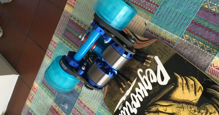
Early 2016 was the year Tesla started showing off their new Model 3 electric car. Unfortunately, my financial situation did not allow me to own such a vehicle. As a result, I settled for the next best thing, building an incredibly overpowered electric skateboard.

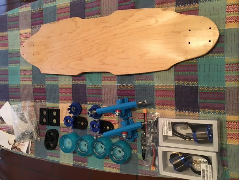
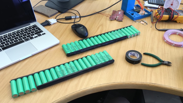
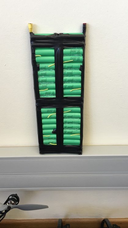
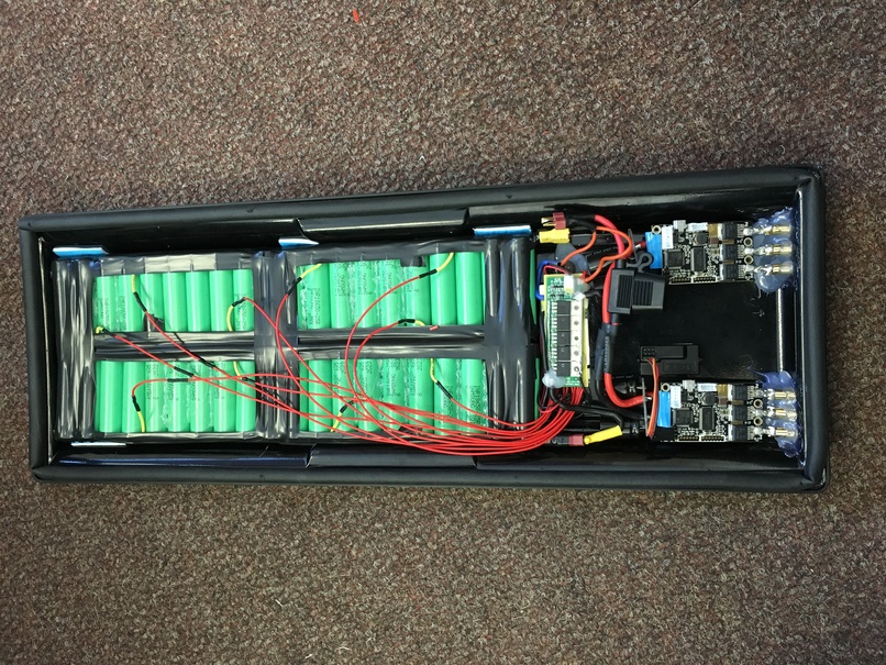
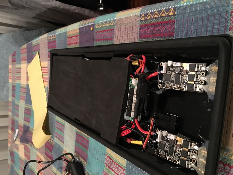
Most of the drive system was ordered as a kit from Enertion (based in Australia). The kit contained dual 6355 brushless dc motors. Both motors were controlled using the popular VESC. The battery was self-assembled out of 40 18650 25R Samsung cells in a 10s4p configuration. I used one of the battery boxes available at Enertion to create a clean build without too much effort. The deck itself was ordered locally.

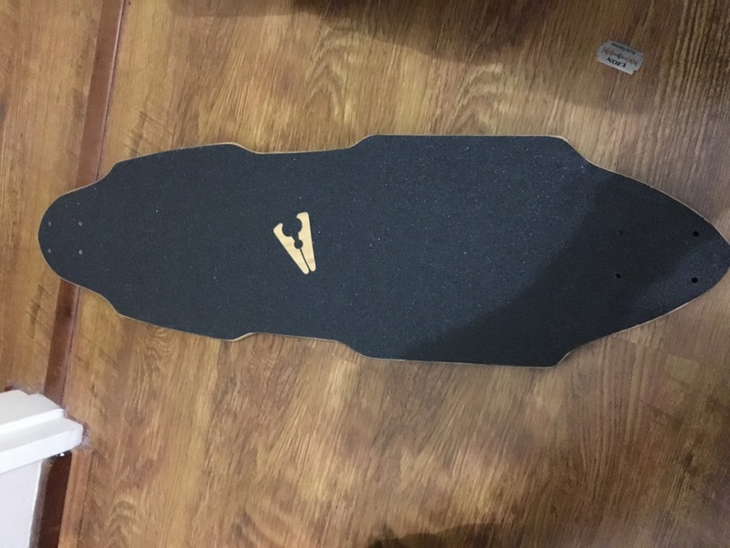
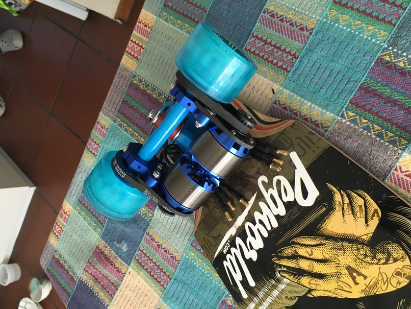
Below are some photos of the build process:

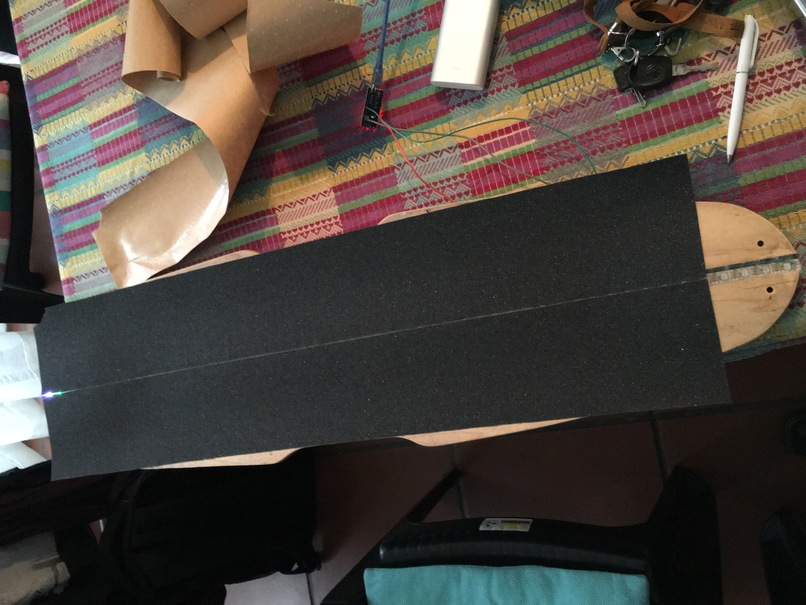
I will be adding some indicator LEDs to the top of the board, so the grip tape had to go.

Assembled drive system

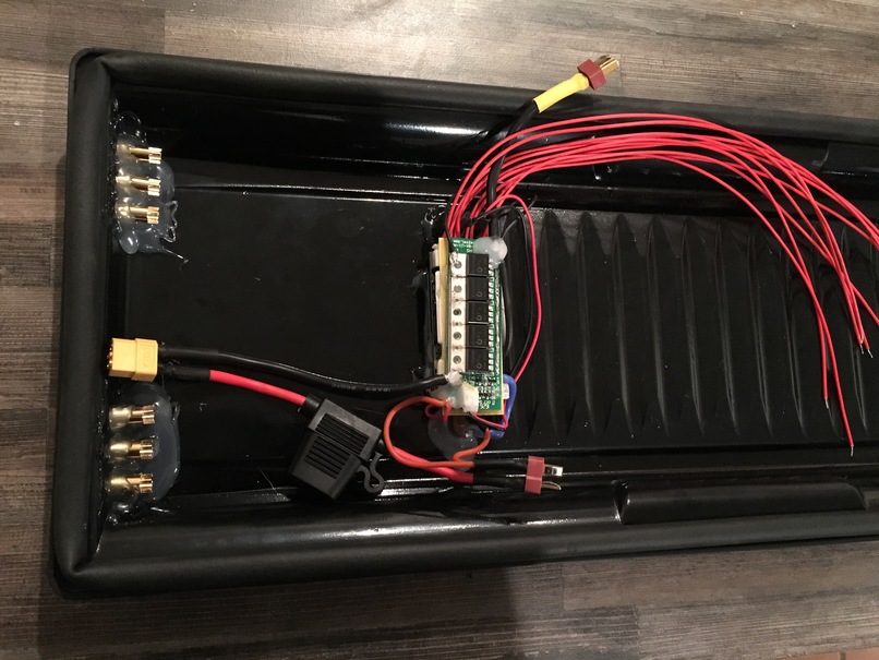
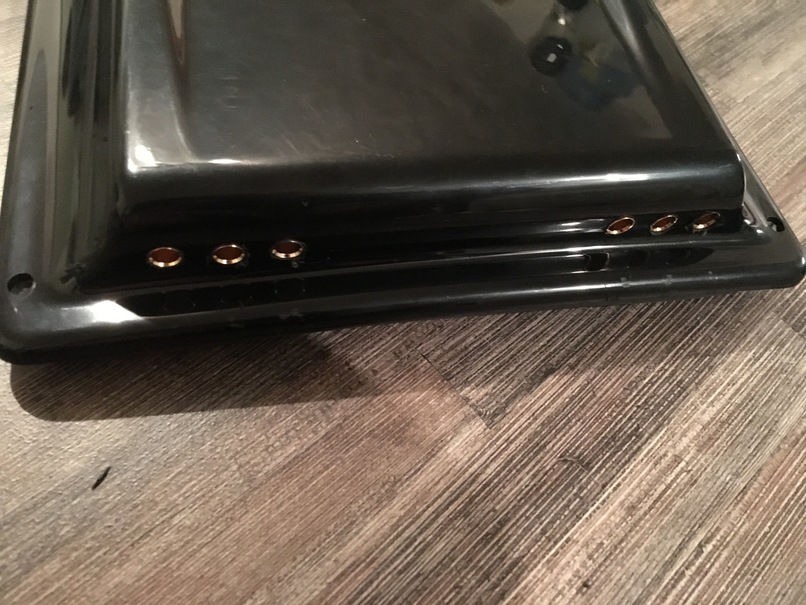
Hot glueing ESC banana-plug connectors in the battery box

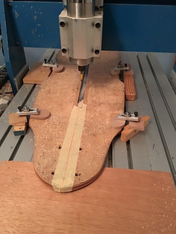
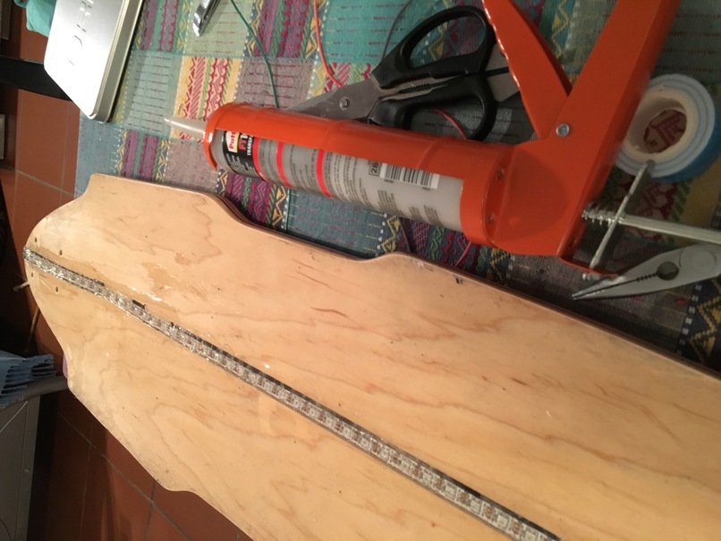
Routing a slot for the neo-pixel LED strip

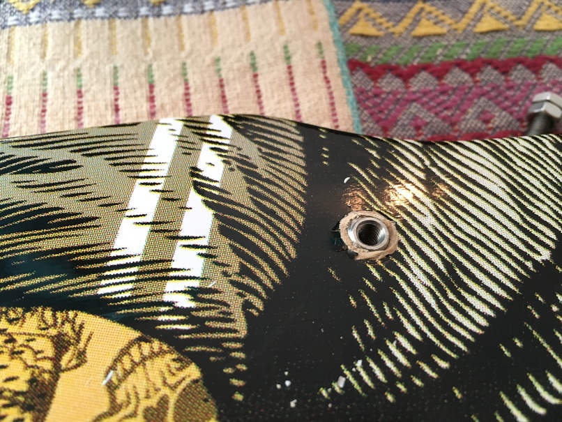
Added inserts to the deck for mounting the battery box

Soldering the Li-ion battery pack

Finished 10s4p Li-ion pack

ESC’s and battery pack installed in battery box

Sealing LED strip using clear silicone

Replacing grip tape, leaving thin slot for LED strip


The LED strip was controlled using an ESP8266. It indicates speed, voltage, current as well as wifi connectivity. The plan was to upload data to a website using an MQTT system. However, excitement took over, and nothing except riding the board was accomplished after this. Since finishing the build, I estimate a total travel distance of more than a 1000 km commuting to and from work. The next post should go into more detail about the LEDs strip with some code and hopefully a working telemetry uploading feature.